The real thing, in the real order. But there are only 69 starting years and they overlap, so a backtest sees just a handful of truly bad decades. The four failures all started between 1965 and 1969.
Monte Carlo Simulation: What It Is and How It Works
A Monte Carlo simulation tests a plan against thousands of possible futures instead of one average. It draws random returns, runs your plan through each sequence, and counts how often the money lasts. That share is the success rate a retirement calculator or a planner shows you.
Take $1,000,000 in a 60/40 portfolio, $40,000 taken out each year and raised with inflation, for 30 years. 896 of 1,000 simulated paths still had money at the end, a success rate of 89.6%. In the 69 real 30-year periods from 1928 to 2025, the same plan lasted 65 times.
The success rate
Paths where the money lasts÷Paths simulated
Each path draws a random return, takes out the spending and moves on, every month for 30 years. 896 ÷ 1,000 = 89.6%.
Simulated, 4% a year89.6%of 1,000 paths lasted 30 years with a 60/40 mix
The other paths104 ran outhalf of them by year 25
History, 1928 to 202565 of 69real 30-year periods lasted at the same 4%
Watch a Monte Carlo simulation run
Every line is one possible 30 years for $1,000,000 paying out a fixed amount after inflation. Start with one path, then add more and watch the success rate settle. Pick a mix and a withdrawal rate to see how they move it.
Paths
Money lastedRan outMedian path
- 1Set the assumptions5.9% ± 12.4%A 60/40 mix of US stocks and 10-year Treasuries returned 5.9% a year after inflation from 1928 to 2025, with 12.4% volatility.
- 2Draw one path360 monthsEach month gets a random return around that average. Path 1 ended its first year at $1,042,786, after the year's spending came out.
- 3Take out the spending$3,333 a monthIt comes out after each month's return. When a withdrawal is due and the balance can't cover it, the path has run out.
- 4Repeat and count896 of 1,000104 paths ran out, so the success rate is 89.6%. The median path ended with $1.65 million in today's money.
Monte Carlo retirement success rates by withdrawal rate
$1,000,000 for 30 years, paying out the first-year rate shown and raising it with inflation. Each row mixes US stocks and 10-year Treasuries, with that mix's own return and volatility after inflation from 1928 to 2025. Pick a cell to run it above.
| Stocks | 3% | 3.5% | 4% | 4.5% | 5% |
|---|---|---|---|---|---|
| 20% stocks3.2% ± 8.4% | |||||
| 40% stocks4.5% ± 9.8% | |||||
| 60% stocks5.9% ± 12.4% | |||||
| 80% stocks7.3% ± 15.7% | |||||
| 100% stocks8.6% ± 19.3% |
Share of 1,000 simulated paths where the money lasted 30 years.
Monte Carlo vs a historical backtest
Three ways to test the same plan: $1,000,000 in 60/40, $40,000 a year after inflation, for 30 years.
Draws every month from the mix's average return and volatility. It builds a thousand new sequences, including worse ones than history has seen, from just two numbers. Our free calculator works this way.
Picks 30 real years at random, with repeats, for each path. It keeps the shape of real returns, crashes included, but breaks up the order they came in. Also called bootstrapping.
Why the order of returns matters
The same 30 years of 60/40 returns, 1966 to 1995, average 4.8% a year after inflation. Taken in order with $40,000 a year coming out, the money ran out in 1991. Taken in reverse, $1.65 million was left. Without any withdrawals, both orders end at $3.30 million.
Retire in 1966, years in orderRan out in year 26
Same years, reversed$1,645,000 left
Balance at each year end in today's dollars, with $40,000 taken at the start of every year. Bars are each year's return after inflation, in order: the first ten compounded at −1.8% a year taken in order and 9.2% reversed. A Monte Carlo simulation draws thousands of different orders, which is how it finds the plans that only fail when the bad years come first.
What is a good Monte Carlo success rate?
Not 100%. A plan that survives every simulated market is usually one that could spend more. Aim for a high score, and know what you'd change if markets disappoint.
Below 80%More than one path in five runs dry. Lower the withdrawal or plan a fallback before relying on it.
80% to 95%T. Rowe Price's confidence zone from age 45 (70% to 95% if you're younger). The 60/40 plan at 4% sits here, at 89.6%.
Above 95%Very safe, and often a sign you're leaving spending on the table. At 3% the same plan scores 97.6%.

T. Rowe Price
Its Retirement Income Calculator runs 1,000 simulations and gives a confidence score. It suggests aiming for a good score rather than a perfect one: 80% to 95% from age 45, and 70% to 95% before that.

Fidelity
Its Retirement Planner runs Monte Carlo simulations and shows results at a 90% confidence level by default: what the plan reached in 90% of simulated markets. It also shows 75% and 50%.
The success rate doesn't say how much is left
A path that ends with $1 counts the same as one that ends with $5 million. Look at the spread of ending balances too. For the 60/40 plan at 4%, half the paths ended above $1.65 million in today's money, and one in four ended with less than $602,000.
5th percentile$0
25th$602,000
Median$1.65M
75th$3.44M
95th percentile$8.17M
What a Monte Carlo simulation leaves out
It's a good tool with known blind spots. Each of these can move the answer more than running more paths.
The inputs decide the answer
The simulation only knows the return and volatility it's given. Assume 4.9% a year for the 60/40 mix instead of 5.9% and the success rate falls from 89.6% to 83.5%.
Random years don't come in runs
Each draw ignores the one before, while real markets have long bad stretches. With 20% stocks at 4%, random draws give 79.6%, but only 43 of 69 historical periods lasted: 10-year Treasuries lost more than half their value after inflation from 1941 to 1981.
Spending never changes
The model keeps taking the same amount after a crash. Spend less in the bad years and fewer paths run out, so read a failed path as a sign the plan needs a fallback, not a forecast that you go broke.
Fees and taxes
They aren't in the returns on this page. A fund charging 0.5% a year takes that straight off the return, so enter a lower return when you run your own plan.
Run a Monte Carlo simulation on your real portfolio
The examples above start from a mix and its history. AllInvestView starts from what you actually hold, across every broker you add.
Portfolio analyzer
1,000 paths from your own holdings
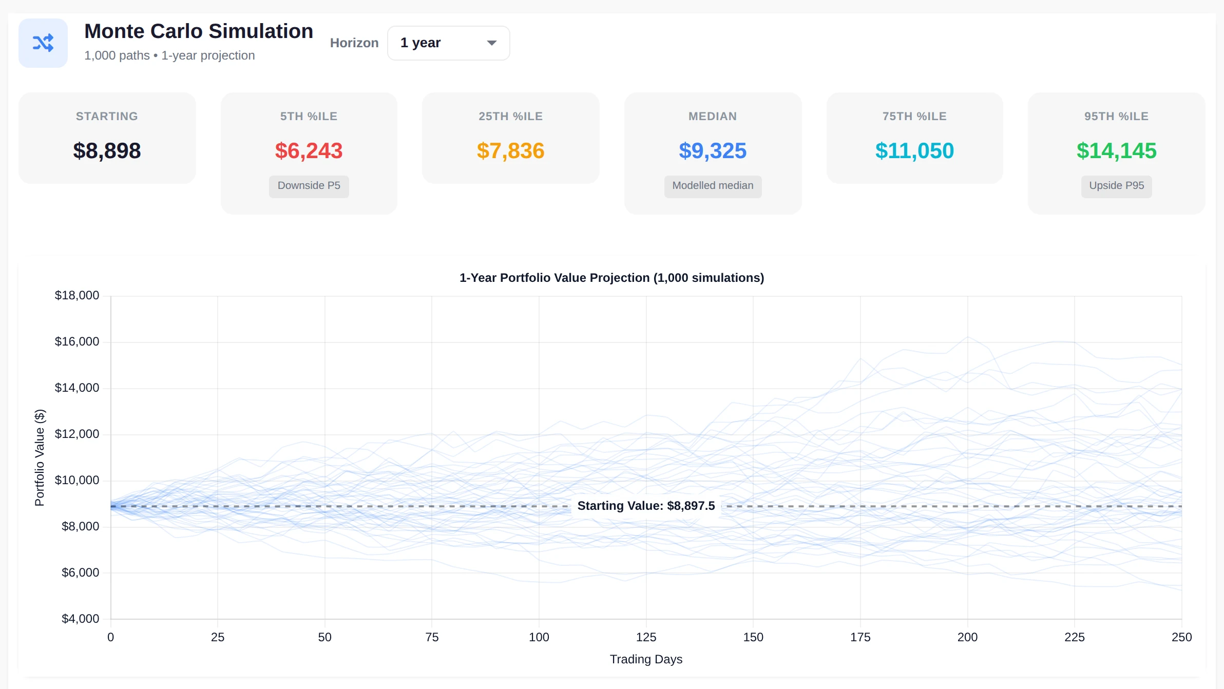
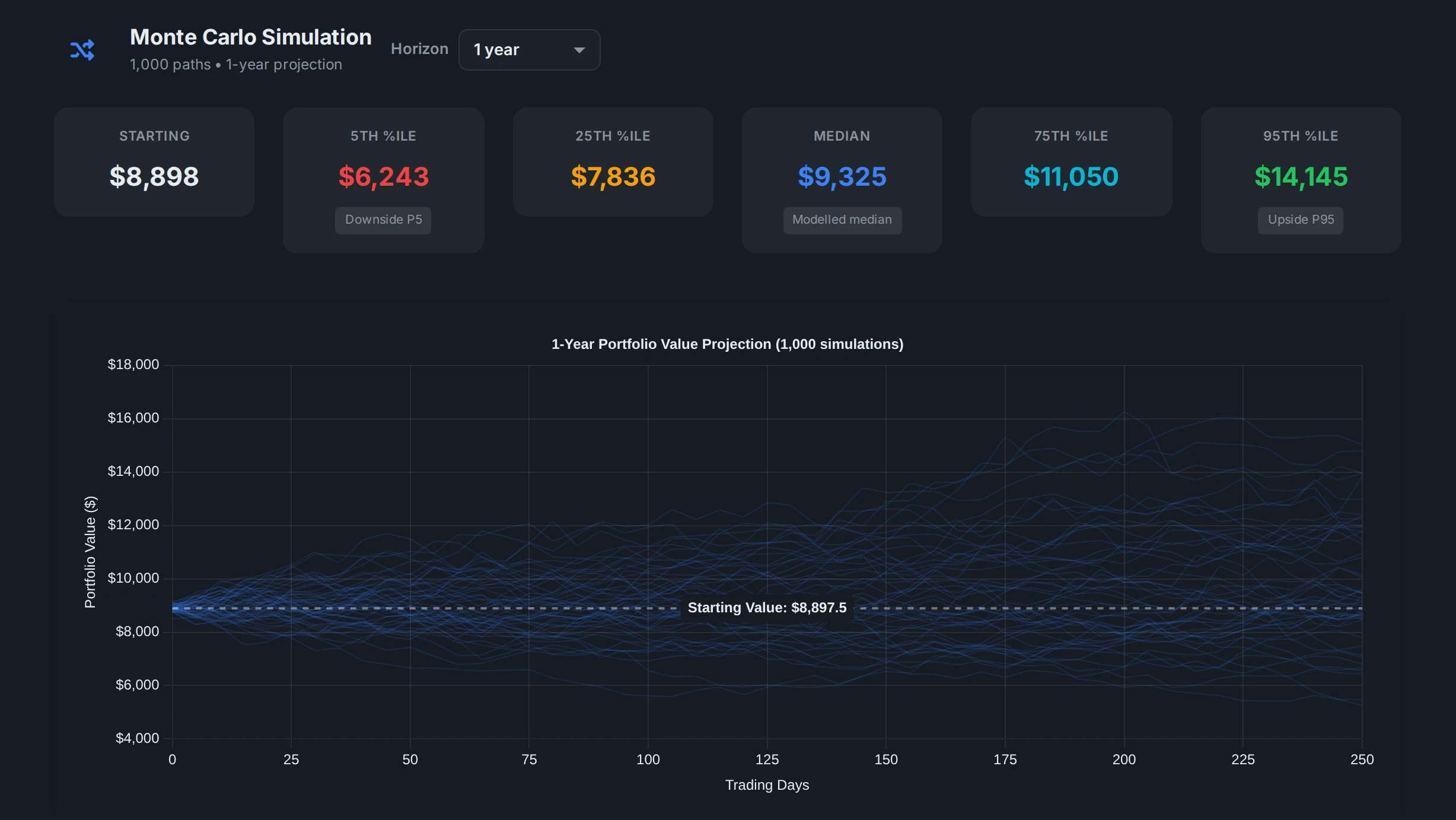
Here the paths come from the holdings you track. Their expected return is set by market risk and their swings by how they really move together, so five tech stocks get a much wider range than a mix of bonds and world funds.
- The 5th, 25th, median, 75th and 95th percentile outcomes, one to ten years ahead
- Next to your efficient frontier, Sharpe ratio, VaR and stress tests
- Holdings kept current through broker sync or a file import
 AllInvestView
Every broker in one place
See a thousand futures for what you actually hold
Add every account you hold and run the Monte Carlo projection, the efficient frontier and stress tests on your real holdings. No spreadsheet of returns to keep up to date.
1,000 paths from your holdings
Efficient frontier, VaR and stress tests
14-day Advanced trial, no card
Questions about Monte Carlo simulation
What is a Monte Carlo simulation in simple terms?
It's a way of testing a plan against many possible futures instead of one. You give it an expected return and how much returns swing, it draws a random sequence of years, runs your plan through it, and repeats that a thousand times or more. The share of runs where the plan works is its success rate.
How does a Monte Carlo simulation work for retirement?
Each simulated path starts with your savings, applies a random return, takes out your spending, and moves to the next period until the end of the plan. A path fails if the money runs out first. $1,000,000 in a 60/40 portfolio paying $40,000 a year, raised with inflation, lasted 30 years in 896 of 1,000 paths: an 89.6% success rate.
What is a good Monte Carlo success rate?
Aim for a high score, not 100%. T. Rowe Price's retirement calculator puts its confidence zone at 80% to 95% from age 45, and 70% to 95% for younger savers. A plan near 100% usually means you could spend more, and one below 80% runs dry in more than one path in five, too often to rely on without a backup plan, like spending less after a bad year.
How many simulations are enough?
A thousand is the usual number and enough for a plan. In the 60/40 example, the first 10 paths gave a 90% success rate, the first 100 gave 88% and all 1,000 gave 89.6%. Running 10,000 gives 90.0%. Assuming a return one point lower moves it far more, to 83.5%.
Is Monte Carlo better than a historical backtest?
It tests more situations. History only has 69 thirty-year periods since 1928 and they overlap, so a backtest sees few distinct bad decades. Monte Carlo builds thousands of new sequences from the same return and volatility. Its weak spot is that random draws miss how real markets cluster: bad years tend to come together.
Does a 90% success rate mean a 10% chance of going broke?
Not quite. It means 10% of the simulated paths ran out under the returns and the spending the model assumed. The model never adjusts. Spend less after bad years and fewer paths run out, so read it as a test of the plan, not a forecast.
Why do Monte Carlo calculators give different answers?
Because the answer depends on what goes in. The expected return, the volatility, inflation, fees, the length of the plan and how spending changes over time all move the result. Assume 4.9% a year for the 60/40 portfolio instead of 5.9% and its success rate drops from 89.6% to 83.5%, so look at the inputs before the score.
Sources
Checked on 24 October 2026.
- Aswath Damodaran (NYU Stern): Historical returns on stocks, bonds and bills, 1928 to 2025, annual returns of the S&P 500 with dividends and the 10-year US Treasury bond, and CPI inflation, updated January 2026.
- T. Rowe Price: How Monte Carlo analysis could improve your retirement plan, June 2026: the Retirement Income Calculator runs 1,000 simulations; its methodology sets the confidence zone at 80% to 95% from age 45 and 70% to 95% before.
- T. Rowe Price Retirement Income Calculator: Methodology, the Confidence Score and the Confidence Zone by age.
- Fidelity Retirement Planner: Detailed methodology, Monte Carlo simulations with a default 90% confidence level, also shown at 75% and 50%.
- William P. Bengen: Determining Withdrawal Rates Using Historical Data, Journal of Financial Planning, October 1994, the historical test behind the 4% rule.
Returns are the S&P 500 with dividends and the 10-year US Treasury bond, less CPI inflation, with each mix rebalanced every year. Simulated paths draw monthly returns from a lognormal distribution whose average matches the mix's yearly return, take the spending out at the end of each month, and use the same 1,000 seeded paths as the calculator. The volatility is applied to the log of each return, which makes the simulated years swing a little more than history did: about 13.2% a year for 60/40 against 12.4%. The historical test and the resampled years take the spending out at the start of each year. None of it is investment advice.